This post is the fourth in my DNN64 series, where I discuss my project of compiling and accelerating deep neural networks (DNNs) on the Nintendo 64 system using modern tools and techniques.
My first post is available here, and the goal is to use modern tools and techniques on this constrained platform.
This post discusses the N64’s co-processor, the RSP, which I am using to accelerate my DNN computations.
The N64’s RSP (Reality Signal Processor) was kind of ahead of its time as a graphics processor.
Although other machines were beginning to include dedicated chips for graphics acceleration, the RSP stood apart as being truly general purpose.
By that, I mean that instead of processing using a small set of fixed functions, it has a full instruction set programmed using assembly.
Its acceleration came from the vector unit, which is a MIPS core with vector instructions (128-bit lanes, with each of the 8 lanes being 16-bits wide).
There is also a scalar unit which can execute simultaneously (assuming there aren’t data hazards), although its instruction set is significantly reduced.
One of the reasons why the project is appealing to me is that this high-level system design, of a CPU with a co-processor with more limited memory, is very similar to modern DNN accelerator environments (CPU+GPU/TPU/etc).
Therefore, many of the design decisions and trade-offs that we will make on this “old” platform are similar to the kind of ones we might make in modern ones.
Namely, how do we fit computations that are too large onto it, balancing the performance considerations of the cost of sending and receiving data, and the fact that we can do work on the CPU at the same time.
Sure, the N64 hardware is old, but these are the same problems I’ve faced in others works using modern hardware, e.g., the SECDA project (led by the talented hardware systems designed Jude Haris).
Moreover, we’re using modern software tooling, so the retro nature of the N64 is almost irrelevant, it’s just in terms of resources it’s now closer to the a contemporary micro-controller.
Kicking it 90s style
One of the first steps I took when looking into this accelerator was to rtfm, if you can believe it.
The RSP manual is available here, released in 1996, which I used to both gain some insights into the RSP’s design and behaviour; as well as some historical interest.
Let’s take a couple of excepts that stood out to me, more on an aesthetic level than a technical one:
For example:
Mastery of the information presented in this document will occur slowly, as
the information is both voluminous and of tremendous breadth. Some
concepts, such as the hardware architecture of the RSP and the microcode
assembly language, are of course thoroughly intertwined; discussion of one
is impossible without the other.
Youch, that doesn’t bode well!
Standing alone, the RSP is an extremely powerful processor; a fixed-point
RISC CPU capable of over half a billion arithmetic operations per second![1]
As part of the RCP, the RSP is an integral part of the graphics/audio/video
processing pipelines.
Recommended background for this chapter includes a solid foundation in
computer architecture, including RISC processors and SIMD (Single
Instruction, Multiple Data) machines.
[1] This is not a misprint. At 62.5Mhz with an 8-element vector pipeline, the RSP could perform 500,000,000 multiply-accumulate operations per second. Since the RSP dual-issues scalar instructions, you could also do another 62,500,000 scalar operations during that same second. That is more than three times the performance of the Cray supercomputers from twenty years ago.
Half a billion arithmetic operations per second!
Can you believe it.
For reference, 2019’s NVidia 3090 can do like five orders of magnitude more!
Although to be fair, both the RSP and the 3090 leave my ability to do mental maths in the dust
This next quote gives information about performance optimization of RSP programs, but also highlights the main designer of the RSP was someone called Mary Jo Doherty.
Mary Jo’s Rules [1]
Avoiding pipeline stalls in software can be accomplished by understanding
the following rules.
VU register destination writes 4 cycles later (need 3 cycles between
load and use). This applies to vector computational instructions,
vector loads, and coprocessor 2 moves (mtc2).
SU register load takes 3 cycles (need 2 cycles between load and
use). This applies to SU loads and coprocessor moves (mfc0,
cfc2, mfc2). SU computational results are available in the next
cycle (see “SU is Bypassed” on page 44).
ny load followed by any store 2 cycles later, causes a one cycle
bubble. Coprocessor moves (mtc0, mfc0, mtc2, mfc2,
ctc2, cfc2) count as both loads and stores.
branch target not 64-bit aligned always single issues.
ranches:
a. Can dual issue (with preceding instruction).
b. o branch instruction permitted in a delay slot.
c. elay slot always single issues.
d. Taken branch causes a 1 cycle bubble.
[1] Named after Mary Jo Doherty, the designer of the RSP.
She seems to have a had a pretty illustrious career, at organisations such as Silicon Graphics (where the RSP was developed), Sun Microsystems, Transmeta Corporation, Digital Equipment Corporation, Oracle, and SambaNova.
Cheers Mary Jo!
Finally, for you hardware-heads, here’s some concise info:
The RSP has a vector processor, implemented as MIPS Coprocessor. The
vector unit (VU) has 32 128-bit wide vector registers (which can also be
accessed as 8 vector slices), a vector accumulator (which also has 8 vector
slices), and several special-purpose vector control registers.
The VU instruction set includes all useful computational instructions (add,
multiply, logical, reciprocal, etc.) plus additional “multimedia instructions”
which are well suited for graphics and audio processing. These instructions
are thoroughly explained in Chapter 3, “Vector Unit Instructions”.
Pipeline depth varies among MIPS processors and their implementations. The RSP has a pipeline depth of 5.
As discussed earlier, the RSP is programmed in assembly, and with a decent enough manual like this, it should be possible to get our accelerated DNN layers implemented this way.
However, writing assembly can be time consuming, and optimizing it has the issue of making it very difficult to parse, especially after multiple passes of optimization strategies like instruction reordering.
In principle, I could write this assembly myself, like my forebears did, but I’m not sure if this is the kind of guy I want to become.
This is one of the many motivations for using a compiler — write your code in a more readable high-level language, and let the compiler handle the generation and optimization of the assembly.
Since LLVM can generate MIPS code, I considered making some alterations specifically for the RSP.
However, this ended up not being necessary because I found as of October 2023, someone is making a DSL (domain-specific language) and optimising compiler for the RSP: RSPL!
RSPL: Really Saves Perry’s Lardon 🥓
I’ve been building up a repository of examples of RSPL, which I’ve released under an MIT License on my GitHub.
I’ll discuss some of these examples more in a future post when I talk about accelerating DNN computations.
You can see some annotated examples below, which I encourage you to copy-paste into the RSPL web-app to see the assembly it generates. Experiment with turning optimization and re-ordering on and off to see its impact:
Add one to a list of 8 values
state{// Allocate space for our datavec16DATA[1];}command<0>AddOne(u32addrData){// first byte of first arg has metadata// that needs to be droppedaddressMatC&=0xFFFFFF;// Perform DMA from CPU into RSP memdma_in(DATA,addrData);// vec16 is a vector type, with 8 16-bit elements// Here we load from RSP mem into a vector registervec16d=load(DATA,0x00);d+=1;// Add one to every element (SIMD instruction)// Store register in RSP memstore(d,DATA,0x00);// Return data to CPU over DMAdma_out(DATA,addrData);}
Reduction of a list of 8 values (sum is stored in idx 0)
command<0>Reduction(u32addressMatC){addressMatC&=0xFFFFFF;// Perform DMA for inputdma_in(INPUT,addressMatC);// Load value into registervec16psum=load(INPUT,0x00);// Use swizzle syntax to get sum// first value is the sum, rest are junkpsum+=psum.yywwYYWW;psum+=psum.zzzzZZZZ;psum+=psum.X;store(psum,INPUT,0x00);dma_out(INPUT,addressMatC);}
Conclusions
This post gave a quick overview of the Reality Signal Processor (RSP), the main accelerator in the N64.
We discussed a little bit about its architecture (128-bit 8 lane vector instructions), as well as how we can program it.
Future posts will discuss how we can accelerate DNN computations using it.
I was delighted to give an invited talk at my alma mater (University of Glasgow) on my DNN64 project, where I have been building an accelerated DNN compiler for the retro N64 console (using modern tools and techniques!)
]]>Perry Gibson 🍐DNN64: An ML Compiler Toolchain for the Nintendo 64 (Part 3) — Activation Maps2024-03-25T11:00:00+00:002024-03-25T11:00:00+00:00https://gibsonic.org/blog/2024/03/25/dnn64_p3
This post is the third in my DNN64 series, where I discuss my project of compiling and accelerating deep neural networks (DNNs) on the Nintendo 64 system.
My first post is available here, and the goal is to use modern tools and techniques on this constrained platform.
This post builds upon the challenges of limited memory discussed in the previous post, with this post looking at the memory requirements of the activation maps.
Previously we spoke about how the N64 only has 4MB of main memory by default, which creates some interesting constraints for any DNNs we want to deploy.
We significantly reduced our memory requirements for the DNN parameters by modifying our code generator such that it stored the weights on disk and loaded them on demand.
This means that instead of loading a full DNN model in one go, we load it partially, and free memory when it is no longer needed.
However, the weights are not the only major contributor to the memory footprint of DNNs.
We also need to think about the activations.
Activations are the actual input data that we pass through the DNN, which are transformed by layers and their parameters.
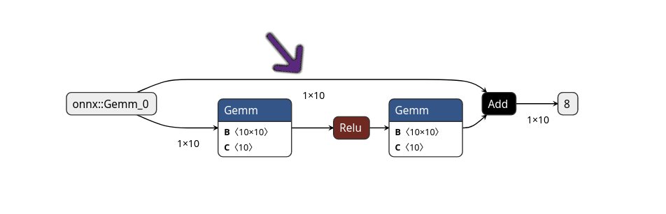
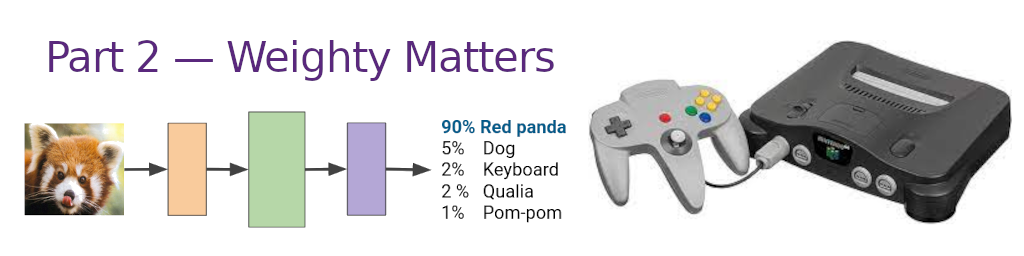
An example of a DNN graph with activations is shown below.
Example of a DNN graph. Nodes are layers (and their weights), and edges are activations. Observe the purple arrow which points at a 1x10 activation matrix.
Ideally we could solve the memory requirements of our activations in a similar way to our weights: only store them for the layer they are required, and free the memory when it is no longer needed.
And in principle, this is what we do.
However, we have a problem: long term dependencies.
In the above graph, observe that there is a branch, where two arrows come out from the first node (onnx::Gemm_0).
This means that the 1x10 activation map is used in both the first Gemm node (bottom branch), and the Add node (where the top branch and bottom branch join).
Therefore we need to store that matrix for a long time, in addition to the other activations generated in the bottom branch.
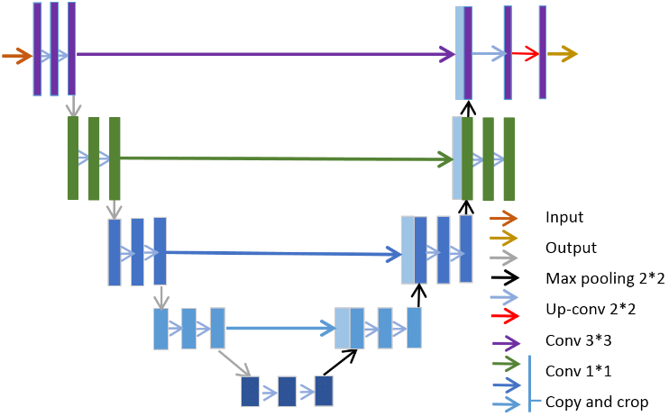
For this trivial network, this isn’t really a problem, but what about for larger DNNs? Take U-Net for example, which has a “U” shape, with lots of very long term dependencies.
Sketch of the U-Net architecture, with many long term dependencies.
With these dependencies, it ends up being very easy to use up all of our available memory, even if the number of parameters at each layer are relatively small.
If we discard the activations in-flight, then we could end up with an incorrect answer.
We have to store these activations somehow until they are consumed.
We could use techniques to reduce the memory required, such as quantisation, or ephemeral sparsity.
But before we think about these techniques, in this post let’s talk about memory planning.
Essentially, we need to consider what the peak amount of “scratchpad memory” we require to store the activations for our model during inference is.
This will be the point where we have the largest memory footprint, potentially storing multiple activation maps.
However, for many DNN architectures there are techniques we can use to reduce this peak, mostly by reordering the execution order of the computation graph.
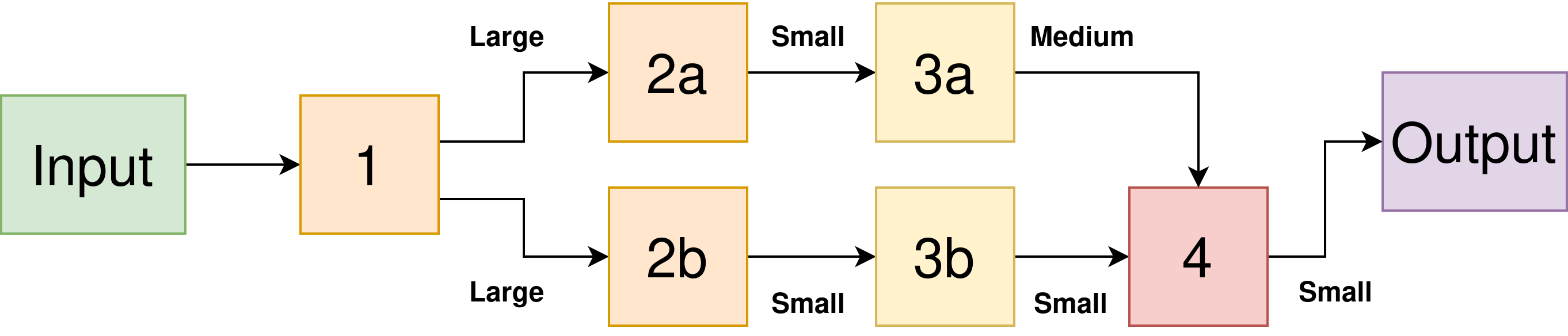
Here’s an example of what I mean — below we have a DNN with a branch and multiple layers.
I’ve labelled the intermediate activations as Small, Medium, and Large.
We have the constraint that we can’t compute a given layer until all of its predecessors have been computed.
But we still have choices of what order to compute the layers.
Can you see how different orderings could give different peak memory requirements?
Diagram showing a branched DNN with activation maps of various sizes.
If we computed the top branch first, then the second, we would compute the layers in the order:
1, 2a, 3a, 2b, 3b, and 4.
However, this has the downside that we need to store the Large activation map generated by layer 1 for a longer time, until it is consumed by our 2b computation.
We also need to store the Medium activation map generated by 3a at the same time, giving us a peak activation memory requirement of Large+Medium.
Instead, a better ordering might be:
1, 2a, 2b, 3b, 3a, and 4.
This means that we can free up the Large activation map sooner, reducing our peak activation memory to Large+Small.
Hopefully that example was reasonably intuitive.
However, for larger arbitrary DNNs the problem is actually quite complex, since we will have many more nodes to consider, and there may be a lot of co-optimization considerations.
It is an NP-hard problem, akin to other scheduling problems such as the bin packing problem.
As a result, it’s tricky to find optimal solutions.
Generally the best we can do is use some heuristics.
At time of writing, Apache TVM (which we are using as the core part of our DNN compiler for the N64) has three main memory planning heuristic algorithms: greedy_by_conflicts, greedy_by_size, and hill_climb. You can see the code for them here, under src/tir/usmp/algo.
Greedy-by-size tries to handle the largest buffers first
Greedy-by-conflict tries to handle buffers which are used by multiple layers first
Hill climb iteratively applies greedy-by-size, trying different permutation orders to find potentially more efficient allocations.
Exploring a variety of DNNs, I found that on average the hill climb algorithm gave me the most compact memory allocation on average, but not in every case.
For example, here is the required workspace for ResNet18 for ImageNet using each of the three algorithms:
Technique
Workspace size (bytes)
greedy_by_conflicts
6909488
greedy_by_size
4818240
hill_climb`
4014080
Ultimately, I’ve found the peak memory of activations to be the main constraining factor for deploying on the N64.
We can load our weights from the cartridge, which can be slow, but at least reduces our memory requirements (almost) as much as possible.
However, since our cartridge is read-only memory, we cannot save our input-dependent activations there.
This means that our peak activations memory cannot exceed 4MB on the N64 (and probably less, since we need memory for our binary and weights).
Sure, we could save long-term activations in some sort of memory card or external storage — the N64 had an accessory called the “Controller Pak” which has 32KB of SRAM.
However that is too small to really help us — our main memory is 4MB afterall, 32KB is almost a rounding error.
In conclusion, intelligent memory planning can save a lot of space for our DNN’s activations and potentially help us fit DNNs which wouldn’t fit on our platform otherwise.
However, this alone won’t be enough in many cases.
Given the strong memory limitation of the N64, we may require additional approaches such as quantisation and ephemeral sparsity to handle our large activation maps and fit larger models.
]]>Perry Gibson 🍐DNN64: An ML Compiler Toolchain for the Nintendo 64 (Part 2) — Weighty Matters2024-03-15T11:00:00+00:002024-03-15T11:00:00+00:00https://gibsonic.org/blog/2024/03/15/dnn64_p2
This post is the second in my DNN64 series, where I discuss my project of compiling and accelerating deep neural networks (DNNs) on the Nintendo 64 system.
My first post is available here.
This post will talk about some of the challenges we face regarding the limited memory of the console compared to the high memory requirements of DNNs, and changes we need to make to our code generator to increase our efficiency and thus increase the size of the models we can run.
In particular, we’ll look at this from the perspective of the DNN weights (also known as parameters).
Weight loading
As discussed in the first post, we’re using MicroTVM to generate C definitions for our DNN.
Let’s take a look at some of the C code generated by an unmodified version of TVM for a simple three layer network.
I’m going to focus on two C files in particular, which should be generated under codegen/host/src, with names like default_lib0.c and default_lib1.c.
The first file contains the main invocation of our DNN:
TVM_DLLint32_ttvmgen_default___tvm_main__(float*dense_4_input_buffer_var,float*Identity_buffer_var,uint8_t*global_const_workspace_0_var,uint8_t*global_workspace_1_var){// constant_X_let are our weight matrices, which we access from the// global_const_workspace_0_var, a contiguous memory region with all our// weights in itvoid*constant_0_let=(&(global_const_workspace_0_var[1216]));void*constant_1_let=(&(global_const_workspace_0_var[1152]));void*constant_5_let=(&(global_const_workspace_0_var[1280]));void*constant_2_let=(&(global_const_workspace_0_var[0]));void*constant_3_let=(&(global_const_workspace_0_var[1088]));void*constant_4_let=(&(global_const_workspace_0_var[1024]));// sid_X_let are our intermediate results, which we store in a workspace// buffervoid*sid_1_let=(&(global_workspace_1_var[96]));void*sid_4_let=(&(global_workspace_1_var[0]));void*sid_7_let=(&(global_workspace_1_var[64]));// We then execute every layer of our model one after another, returning 0 if// the execution was successful. Our output should be stored in// Identity_buffer_varif(tvmgen_default_fused_reshape(dense_4_input_buffer_var,sid_1_let,global_const_workspace_0_var,global_workspace_1_var)!=0)return-1;if(tvmgen_default_fused_nn_contrib_dense_pack_add_nn_relu(sid_1_let,constant_0_let,constant_1_let,sid_4_let,global_const_workspace_0_var,global_workspace_1_var)!=0)return-1;if(tvmgen_default_fused_nn_contrib_dense_pack_add_nn_relu_1(sid_4_let,constant_2_let,constant_3_let,sid_7_let,global_const_workspace_0_var,global_workspace_1_var)!=0)return-1;if(tvmgen_default_fused_nn_contrib_dense_pack_add(sid_7_let,constant_4_let,constant_5_let,Identity_buffer_var,global_const_workspace_0_var,global_workspace_1_var)!=0)return-1;return0;}
As you can see, we prepare pointers to our weight and activation arrays first (e.g., *constant_0_let and *sid_1_let respectively), then run each layer of our DNN.
These buffers are prepared in the other C file:
// Our workspace, comprised of 160 bytes__attribute__((section(".bss.noinit.tvm"),aligned(8)))staticuint8_tglobal_workspace[160];// Our weight arrays, in hex format__attribute__((section(".rodata.tvm"),))staticstructglobal_const_workspace{floatconstant_2_let[256]__attribute__((aligned(16)));// 1024 bytes, aligned offset: 0floatconstant_4_let[16]__attribute__((packed,aligned(16)));// 64 bytes, aligned offset: 1024floatconstant_3_let[16]__attribute__((packed,aligned(16)));// 64 bytes, aligned offset: 1088floatconstant_1_let[16]__attribute__((packed,aligned(16)));// 64 bytes, aligned offset: 1152floatconstant_0_let[16]__attribute__((packed,aligned(16)));// 64 bytes, aligned offset: 1216floatconstant_5_let[1]__attribute__((packed,aligned(16)));// 4 bytes, aligned offset: 1280}global_const_workspace={.constant_2_let={-0x1.4a62b2p-2,-0x1.8c75ap-3,-0x1.4457fp-5,0x1.ee096ap-3,-0x1.aa9a3ep-3,0x1.4e7fd4p-2,0x1.22d84ep-2,-0x1.fcbcep-5,// and so on},.constant_4_let={-0x1.34a976p-1,-0x1.f681e2p-1,0x1.0a4db6p-1,0x1.315aeep-1,0x1.bb42f6p-1,0x1.874a72p+0,// and so on},// our other weight arrays get assigned their values.constant_5_let={-0x1.928ffp-2},};// of total size 1284 bytes
As you can see, we are hard coding the weights in this C file, meaning they will be compiled into our executable.
We can then access them via the pointers we initialised in our main function.
All very well and good, but we have a problem.
If we try and compile a larger model, our individual object files are generated correctly, but we get a linker error, for example:
/opt/libdragon/bin/../lib/gcc/mips64-elf/13.2.0/..////mips64-elf/bin/ld:
region men' overflowed by 132146288 bytes

collect2: error: Id returned 1 exit status

make: (Makefile:46: build/dnn64.elf] Error 1
What’s happening here?
Clearly we are running out of memory — the N64 only has 4MB afterall — but why is this happening, shouldn’t MicroTVM be optimised for microcontrollers?
To answer this question we need to talk briefly about ELF files and linker configuration.
ELF 🧝 and (lib)dragon 🐉
You might have noticed this snippet in our weight definition code section(".rodata.tvm").
This is to indicate to the compiler that this is “read-only data”, and should be placed in the appropriate part of the ELF file.
But what is an ELF file?
Standing for Executable and Linkable Format, ELF files are a standard format for executable programs, especially in UNIX-like environments.
It defines where and how our executable code is stored, along with any data it requires, and metadata that can be used to help interpret it correctly.
It’s the format used by the N64, all of the Sony PlayStations, Linux, FreeBSD, Fuchsia, and more.
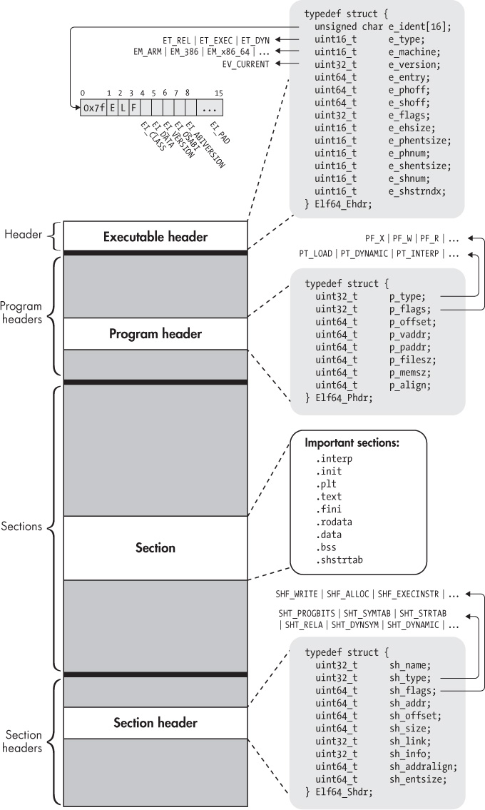
Below is a diagram showing the main components and structure of an ELF file, to give you an idea of what that looks like:
High-level structure of the ELF format (diagram source here). Note in particular that we have different sections, e.g., .init, .text, .rodata, .bss.
And here’s a more detailed diagram of how it’s structured, from Ange Albertini. If you’re interested in learning more, the ELF Format Cheatsheet gives some great information.
When we compile our program, we may have multiple object (.o) files, that we must combine together to get our final executable.
It is the linker’s responsibility to combine them together in a coherent way to form an ELF file.
Let’s poke around our linker configuration file for the N64 to understand what is happening.
/* Start address of code is 1K up in cached, unmapped RAM (KSEG0). We have
* to be at least this far up in order to not interfere with the cart
* boot code which is copying it down from the cart
*/__libdragon_text_start=__kseg0_start+0x400;MEMORY{mem:ORIGIN=__kseg0_start,LENGTH=4M}SECTIONS{// Our sections, which we'll get to in a moment
You’ll notice the MEMORY definition, where we define one region of memory, which is 4MB, corresponding to the N64’s memory.
If our linker finds that it requires more than this for our program, then it will crash with an error.
Let’s look at the SECTIONS definition too:
SECTIONS{/* The text section carries the app code and its relocation addr is
* the first byte of the cart domain in cached, unmapped memory
*/.text__libdragon_text_start:{*(.boot).=ALIGN(16);__text_start=.;*(.text)*(.text.*)*(.init)*(.fini)*(.gnu.linkonce.t.*).=ALIGN(16);__text_end=.;}>mem.eh_frame_hdr:{*(.eh_frame_hdr)}>mem.eh_frame:{__EH_FRAME_BEGIN__=.;/* Define symbol for accessing eh_frame section */KEEP(*(.eh_frame))}>mem.gcc_except_table:{*(.gcc_except_table*)}>mem.jcr:{KEEP(*(.jcr))}>mem.rodata:{*(.rdata)*(.rodata)*(.rodata.*)*(.gnu.linkonce.r.*).=ALIGN(8);}>mem/* This is important to keep __CTOR_END__ consistent */.=ALIGN(4);// other sections
You’ll note that our .rodata (read-only data, including our DNN weights) is being stored in mem, so if they exceed 4MB then our linker will crash.
It’s difficult to find a DNN with less than 4MB of weights, so this is going to be a problem.
Why does MicroTVM store the weights in the ELF file like this, when it’s targeting memory constrained microcontrollers?
The reason for this is demand paging.
In newer systems, especially in memory constrained environments, the OS is often configured to only load data as it is required (pages at a time).
This means that for most of the microcontrollers that MicroTVM targets, it doesn’t load all of the weights at once.
Instead, they will be kept in the storage medium, and when a piece of code access that range of the weight array, the OS will load that page of data, and free it when it is not needed.
Unfortunately, the N64 does not really have a concept of demand paging like this.
We’re actually programming on bare metal, and we need to embed a small OS into our .z64 file.
Therefore, in the case of the N64, we load the entire ELF file into memory at once, and if it that’s more than 4MB, our linker file won’t generate it.
But hold on a second! You’ll recall in the first post that the N64 has unified memory.
One thing that means is that our cartridge (our storage medium for our game) is memory mapped, and thus addressable.
The cartridge can hold much more than our memory, potentially hundreds of MBs.
Could we edit our linker script so that we store our .rodata on the cartridge region of memory, rather than the main memory region?
Yes!
Let’s just add a new section to MEMORY called cartridge, and store our .rodata on it.
As you can see on this page of the N64brew wiki, the cartridge region of memory starts at 0x10000000.
But because of the way addressing works on the N64 (even though we have a 64-bit addressing mode, most programs address in 32-bit), we need to use a translation.
MEMORY{mem:ORIGIN=__kseg0_start,LENGTH=4Mcartridge:ORIGIN=0x00000000,LENGTH=32M/* Adjust to actual cart size *//* cartridge : ORIGIN = 0x10000000, LENGTH = 32M */}SECTIONS{// rest as previous.rodata:{*(.rdata)*(.rodata)*(.rodata.*)*(.gnu.linkonce.r.*).=ALIGN(8);}>cartridgeAT>mem/* note we are storing in a new place now */
Great, this looks like it could work, meaning we can now fit an (almost) arbitrary number of weights in our program, since they are stored in the cartridge.
However, let’s take a step back and think about what would be happening here…
Our weights are now stored in the cartridge region.
So if we access constant_0_let[0], instead of loading it from main memory we fetch it from cartridge.
And this is super slow, and will thus be unacceptable for our DNN inference application.
Repeated accesses may also be slow, since there’s no guarantee that our arrays will be cached.
Do you remember loading screens in video games?
This is what they were for, and oh boy do we not want to have one for every parameter we load.
Accessing data from the cartridge on-demand is not workable — the latencies are too high.
Instead we should copy the data to main memory when it is needed, and free it when we are done with it.
If we had some sort of demand pager that copied the arrays over to main memory when required, then we could fix the performance issue we have introduced.
However, 1. this would be a relatively complex system to implement, 2. I’m lazy (in the pragmatic way!), and 3. we know the access patterns to our weights ahead-of-time.
Perhaps there’s a simpler solution?
The answer is yes: weight serialisation.
By saving our weights as files, we can store them on our cartridge, and load them into memory when required.
Libdragon has a great little filesystem implementation for just this purpose.
A simple loading schedule would be to load them just before we execute the layer that requires them, and free them when the layer has been executed.
But a more advanced schedule would load the maximum amount of weights we can fit in 4MB, and hide the loading latency by loading new weights asynchronously.
Let’s look at how we would implement this.
Implementing just-in-time weight loading
Code generation
Our end state should be an extension to our code generator, such that it produces something like the below function, where we load and freeing the weights from file before they are required in a given layer.
TVM_DLLint32_ttvmgen_default___tvm_main__(float*dense_4_input_buffer_var,float*Identity_buffer_var,uint8_t*global_const_workspace_0_var,uint8_t*global_workspace_1_var){// constant_X_let are our weight matrices, which we access load from// the cartridge, a contiguous memory region with all our weights// in itvoid*constant_0_let;// forward declaration of weightsvoid*constant_1_let;void*constant_5_let;void*constant_2_let;void*constant_3_let;void*constant_4_let;// sid_X_let are our intermediate results, which we store in a workspace// buffervoid*sid_1_let=(&(global_workspace_1_var[96]));void*sid_4_let=(&(global_workspace_1_var[0]));void*sid_7_let=(&(global_workspace_1_var[64]));// We then execute every layer of our model one after another, returning 0 if// the execution was successful. Our output should be stored in// Identity_buffer_varif(tvmgen_default_fused_reshape(dense_4_input_buffer_var,sid_1_let,global_const_workspace_0_var,global_workspace_1_var)!=0)return-1;if(read_file_into_memory("rom:/constant_0_let.dat",&constant_0_let)!=0)return-1;if(read_file_into_memory("rom:/constant_1_let.dat",&constant_1_let)!=0)return-1;if(tvmgen_default_fused_nn_contrib_dense_pack_add_nn_relu(sid_1_let,constant_0_let,constant_1_let,sid_4_let,global_const_workspace_0_var,global_workspace_1_var)!=0)return-1;freeconstant_0_let;freeconstant_1_let;if(read_file_into_memory("rom:/constant_2_let.dat",&constant_2_let)!=0)return-1;if(read_file_into_memory("rom:/constant_3_let.dat",&constant_3_let)!=0)return-1;if(tvmgen_default_fused_nn_contrib_dense_pack_add_nn_relu_1(sid_4_let,constant_2_let,constant_3_let,sid_7_let,global_const_workspace_0_var,global_workspace_1_var)!=0)return-1;freeconstant_2_let;freeconstant_3_let;if(read_file_into_memory("rom:/constant_4_let.dat",&constant_4_let)!=0)return-1;if(read_file_into_memory("rom:/constant_5_let.dat",&constant_5_let)!=0)return-1;if(tvmgen_default_fused_nn_contrib_dense_pack_add(sid_7_let,constant_4_let,constant_5_let,Identity_buffer_var,global_const_workspace_0_var,global_workspace_1_var)!=0)return-1;freeconstant_4_let;freeconstant_5_let;return0;}
How can we achieve that?
First, let’s dump the weights of our DNN to file.
Before we automate this in our codegen stage, I wrote a wee Python script to parse our generated .c file.
You can see it on this gist, but it isn’t necessary to read it.
All it does is convert our weight arrays to binarised .dat files, which can be loaded by our C program.
We also generate a .csv file for manual visual inspection.
But we don’t use this in our program, since parsing the raw text of a CSV would be more expensive than loading binary data.
Next, we must figure out where in our code generation pipeline to insert our loading and freeing code.
Like most compilers, TVM represents its computation as an AST (abstract syntax tree), and then translates that to the appropriate format for the chosen backend.
For our C backend, this it the CodeGenC class, in target/source/codegen_c.[cc/h].
This subclasses CodeGenSourceBase, and inserts the appropriate C code given its walk of the AST.
For example, here’s how it handles generating the code for a while loop.
voidCodeGenC::VisitStmt_(constWhileNode*op){PrintIndent();// Adds indentations to our source filestream<<"while (1) {\n";// We are just printing our C to an output streamintwhile_scope=BeginScope();std::stringcond=PrintExpr(op->condition);PrintIndent();stream<<"if (!("<<cond<<")) { break; }\n";PrintStmt(op->body);// Our body can be arbitrary, so other VisitStmt_ may// be called before we return from herethis->EndScope(while_scope);PrintIndent();stream<<"}\n";}
We want to preserve all of this functionality, but have a special case for loading our weights when we are in the main function.
We can check if we are in the main function by editing the AddFunction method.
Our assignments (e.g., void *constant_0_let = (&(global_const_workspace_0_var[1216]));) are generated when handling LetStmtNodes.
But we don’t want to completely replace it, since we only want this behaviour in our main function for our weights, and leave the default behaviour otherwise.
We could subclass CodeGenC, but instead I’m going to use a “State” design pattern (discussed here).
This is where we switch out the implementation for a given subset of our class’s functions with a state change.
Most of the time we will use the original implementation, but if we are generating the main function we use a different one.
Crucially, any visits we do to subsequent nodes of types other than LetStmtNode will still use the original version (unless we also override them).
I’ll discuss the tradeoffs of using this pattern versus just subclassing when I try and upstream this feature into TVM.
I chose it here because it was easier to implement.
We could have some code generation look something like:
voidDefaultVisitorState::VisitStmt_(constLetStmtNode*op,CodeGenC*codegen){// Original code}voidMainFuncVisitorState::VisitStmt_(constLetStmtNode*op,CodeGenC*codegen){// For our weight arrays, instead of printing to a stream,// store in std::unordered_map<std::string, std::string> load_var_code_// where the key is the var_name. We will print later// we will store our code for later use// Workspace accesses are printed as normalauto&var_idmap_=codegen->var_idmap_;auto&handle_data_type_=codegen->handle_data_type_;std::stringvalue=codegen->PrintExpr(op->value);std::stringvar_name=codegen->AllocVarID(op->var.get());std::stringdtype="void";std::ostringstreamstream;// misc codestream<<" static "<<dtype;stream<<"* "<<var_name<<"; // Declare without immediate initialization \n";// Open file to read binary datastream<<" if (read_file_into_memory(\"rom:/"<<var_name<<".dat\", &"<<var_name<<") != 0) return 0;\n\n";load_var_code_[var_name]+=stream.str();}
If we were to just print to our regular output stream, we would have a problem, namely because of the structure of the AST, all of the loads are generated when the variables are defined — before any of our computation occurs.
This defeats the purpose of our lazy-loading structure, and we wouldn’t save any memory.
Instead, we should generate code for our variable declarations, and generate our loading code later (saved in a map/dictionary load_var_code_).
Using our simple scheduling, we will generate that code right before we require the given weight array for a layer invocation.
Our layer invocation code is generated in VisitStmt_ for CallNodes.
Let’s inject our array loading code before the invocation, and our free statements afterwards.
Note that we need to inspect the variables used by the layer invocation to identify what load and free code we should generate.
So something like:
// Target example// if (read_file_into_memory("rom:/constant_0_let.dat", &constant_0_let) != 0) return -1;// if (tvmgen_layer(// sid_1_let, constant_0_let global_const_workspace_0_var,// global_workspace_1_var) != 0)// return -1;// free constant_0_let;constCallNode*call=op->args[2].as<CallNode>();if(main_state)main_state_->LoadArrays(call,this);// load any arrays that might be neededos<<"if (";VisitExpr_(call,os);os<<" != ";PrintExpr(op->args[0],os);os<<" ) return ";PrintExpr(op->args[1],os);if(main_state){// free any arrays that we don't needos<<";\n";main_state_->FreeArrays(call,this,os);};
And with that, our code is being generated correctly, matching our target at the top of this section.
Weight serialisation
Now that we are generating our code correctly, we should add a step to automatically serialise our weight arrays to file in our compiler, rather than having to do it manually.
The part of TVM responsible for exporting our weights is target/source/source_module.cc.
To extend this with dump-to-file capabilities, we should really add a compilation flag (e.g., serialize_weights), but I’m just going to comment out the original functionality.
TVM represents the weights as an NDarray object, which stores information on the number of elements, the shape, and the data type.
The code for this could be something like:
voidGenerateBinarisedArray(conststd::string&name,construntime::NDArray&array,int64_tnelems){std::vector<float>out_data(nelems);array.CopyToBytes(out_data.data(),nelems*sizeof(float));// Save the data to a filestd::stringfilePath="./filesystem/"+name+".dat";std::ofstreamoutFile(filePath,std::ios::binary);if(!outFile){std::cerr<<"Cannot open file for writing: "<<filePath<<std::endl;return;}// Write to filefor(floatvalue:out_data){char*floatToConvert=reinterpret_cast<char*>(&value);outFile.write(reinterpret_cast<constchar*>(&value),sizeof(float));}outFile.close();}
Remember, we also need to remove the code generation for the .rodata allocations of the weight arrays, otherwise we won’t save any memory.
Now, our compiler should now do everything we need to implement the lazy weight-loading system!
A fun bug
But there’s just one issue.
Our weights should look like this:
What could be happening, why are they different?
Is there a bug in our weight file loading code, or our serialisation?
It doesn’t seem like it — if we run the loading code as a standalone C program on my laptop, using the exact .dat files, then we get the correct output.
So what’s happening?
Why is the N64 interpreting this data differently?
I’ve spoiler tagged the answer, because I think it’s mildly interesting, and can be worked out from the information I’ve given you already.
Click to reveal the answer
The answer is endianness!
Most modern machines (including x86 and ARM) default to a little-endian representation of data.
However, the N64 with its MIPS CPU uses a big-endian format.
That means that it is reading our bytes for a given element in reverse order.
So it would read the little-endian number 0000 0011 0111 1111 as 0111 1111 0000 0011.
This explains why our small numbers on the laptop are large when loaded on the N64.
By reversing the order of the bytes on our export we now get the correct outputs!
Conclusions
This post outlines how we can overcome the 4MB limit of the N64 when running large DNNs by storing the weights as binarised files on our cartridge, and only loading them when needed.
The original design of our compiler assumed that we had access to some sort of OS level demand paging for ELF files, but to date no such functionality exists for the N64.
Therefore we generate the code to do this ourselves.
Note that we rely on the filesystem utilities available in Libdragon, which is why we prepend our paths with rom:/.
We need to enable this feature in our Makefile, so it knows to copy over any of our .dat files into the .z64 cartridge files we generate.
You can see an example of working with the Libdragon filesystem here.
As discussed above, we could further optimise this feature by being more intelligent with our weight loading schedule, and doing so asynchronously.
This solution is almost space optimal — we only load weights when they are required, but it isn’t time optimal.
But for now, it’s good enough that we can now generate working code for larger models on the N64.
The only way we could get more space optimal would be to load partial weight arrays, but that would be a more complex scheduling problem.
In the next post, we’ll discuss the issue of the memory requirements of the intermediate activations.
For now, catch ye.
]]>Perry Gibson 🍐DNN64: An ML Compiler Toolchain for the Nintendo 64 (Part 1)2024-03-12T11:00:00+00:002024-03-12T11:00:00+00:00https://gibsonic.org/blog/2024/03/12/dnn64_p1
In the first of a series of blogposts, I discuss my experience developing and accelerating a compiler toolchain for running deep neural networks on the Nintendo 64 (1996).
I endeavoured to use modern tools (e.g., Apache TVM), and acceleration techniques which are relevant to today’s models and hardware accelerators.
But of course there will be special considerations required to fit them to the unique hardware and software environment of this beloved (by some, it was out before I was born) games console.
This first post will give an overview of my system design, and future posts will go deeper into individual challenges (in ML, compilers, and hardware).
I’m interested in tensor compilers, especially those for deep neural networks (DNNs).
One attractive feature of many of them, compared to hand-written kernel libraries such as cuBLAS, is that you can take a given program as input and generate code for multiple different hardware and software backends.
One thing I’ve wondered for a couple of years is how easy it would be to get a modern DNN working on retro hardware, especially games consoles.
Some like to market DNNs as the hot new thing, but they’re an old idea, its just recently that the availability of large datasets and powerful hardware has made them more practical and scalable.
The training of these networks is the most compute intensive part, with inference (i.e., deploying a trained model) being relatively cheap — though still important to optimise when running at scale.
Could we run a pre-trained DNN on, for example, a machine older than me?
Hence, this project was born: DNN64, where I try and run (and hopefully accelerate!) DNNs on the Nintendo 64 games console.
I don’t yet have access to real N64 hardware, but luckily there is a dedicated community of folk who develop emulators for it, such as ares,
cen64, dgb-n64,
simple64.
There’s even an FPGA emulator pretty far in development!
Kudos to them, as it serves an important public good of ensuring that the cultural artefacts of these games will still be archived and usable long after the last N64 has broken down.
My initial development will be in these emulators, and if any of my pals have a real N64 in their attic somewhere, I’d love to try and run there too.
I’m going to structure this first post introducing the core components of my solution (the N64 toolchain, the N64 hardware, Apache TVM, and how we bring it all together), as well as the challenges we face regarding acceleration. Future posts will discuss how those challenges are tackled, as well as my efforts towards optimisation.
For the record, I have no experience with game console emulation and retro homebrew development — I came at these topics as an outsider.
Please get in touch if you spot any errors!
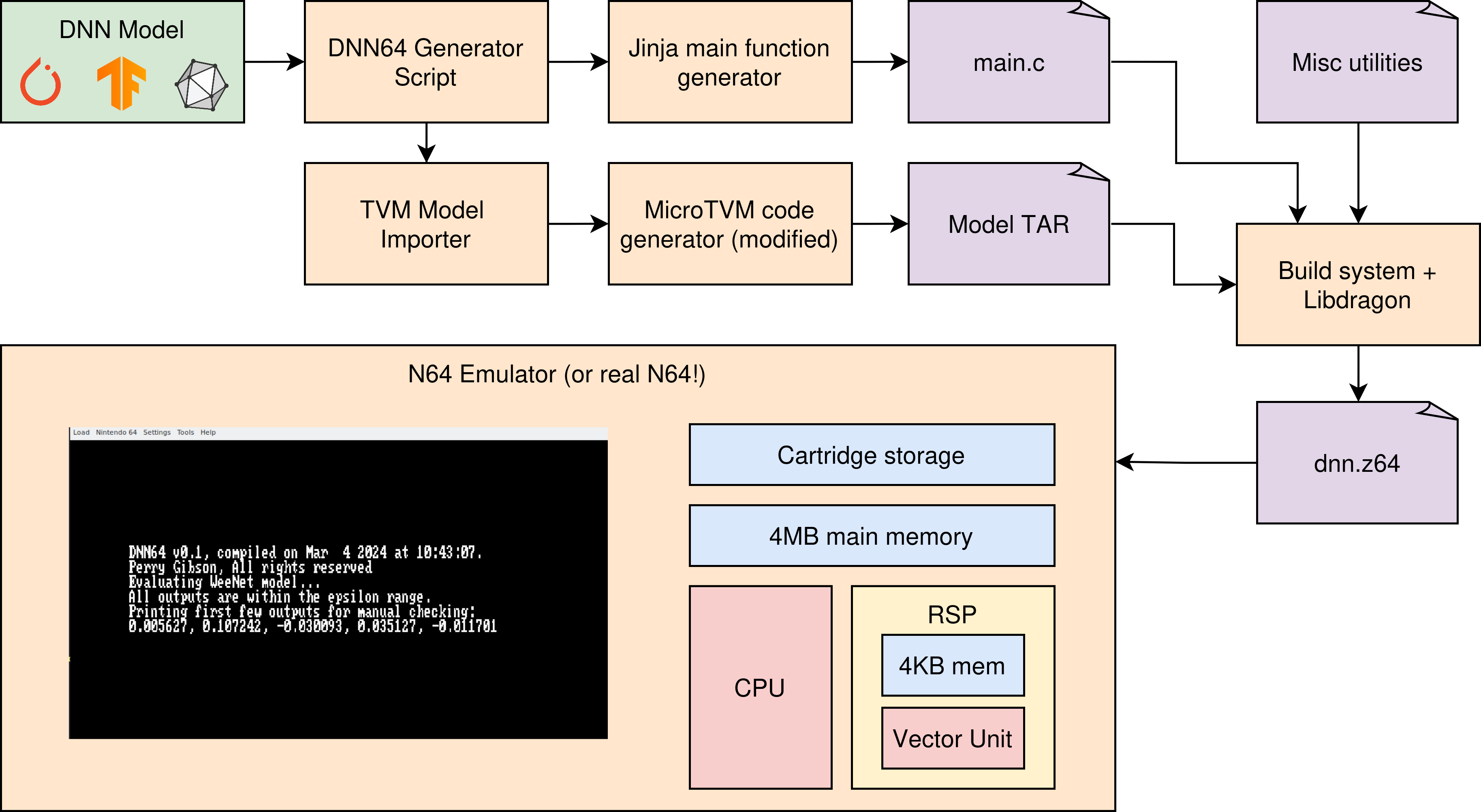
At a high level, you can see a sketch of my system in the below figure.
I hope that this series of posts will help make clear the relevant components, how I desgined and implelemented them, and my strategies for optimisation.
High-level overview of DNN64. The user inputs a DNN model from a framework of their choice, and an N64 executable file (`dnn.z64`) is generated.
The N64 toolchain
Back in the 1990s, folk typically programmed for the N64 in assembly and C.
Nintendo sold an official development kit called Ultra64, and some folk still develop using that (both legal and pirated copies).
As an aside, I recall hearing that Super Mario 64 was one of the first titles that Nintendo developed using C, and for the original Japanese release, reverse engineers have discovered that they didn’t enable compiler optimizations (i.e., with -o2 or higher).
It’s a testament to their rigour that it runs as well as it does, except for a couple of corners exploited by speedrunners.
We have two main options for our project: either we program in C and use an existing N64 compiler toolchain, or we get another toolchain (say TVM) to generate code for the N64’s ISA directly.
I’ve gone for the C approach, but don’t despair compiler heads, I’ll be using a compiler to generate C!
The reason for this is that there will be a lot of hardware knowledge represented in the configuration on an existing N64 compiler toolchain — I don’t relish the thought of trying to reproduce it all in LLVM, and be ABI compliant if I want to integrate with other tools such as those for showing graphics.
First, I tried compiling a modern version of gcc to generate code for the N64’s MIPS CPU architecture (discussed more in the next section).
This was going off of this WikiBooks page on N64 development
See my post on other gcc build issues you might encounter if you go down this route.
However, the next steps of creating an N64 ROM cartridge (typically distributed as .z64 files) from my binary had a few too many steps.
Given that is was getting cumbersome, I looked further afield for a more specialised toolchain, ideally with an active community.
Next, I found a pre-configured N64 toolchain n64chain, which seemed to provide some of this functionality.
It seemed great, however it was missing one critical piece of code required — the boot code, for booting up the system.
This is copyrighted, and not distributed by the authors of n64chain for obvious reasons.
Fortunately, it appears that folk have been able to make open source versions of the boot code, and also exploit hash collisions in the N64’s checksum to allow it to be accepted by the console.
More details of that are given here.
My adventure into finding a legal and functional boot code let me to the libdragon SDK, which includes open source boot code, as well as a lot of other quality-of-life tooling for N64 development.
Therefore, I opted to use this for the DNN64 project, and I’ve not looked back.
Libdragon builds off of a modern version of gcc, but provides N64-appropriate build configurations to make it easier to generate that coveted .z64 file which actually works.
It makes it straightforward to include C standard library functions, and provides its own utilities for things such as 2D graphics programming (with a port of OpenGL for 3D graphics under development!), debugging, audio, and data management.
I’ll be packing up my full workflow for DNN64 at a later date, but if you’re interested in getting started with libdragon, I would recommend the containerised CLI, at least for your initial steps.
The N64 hardware
Now that we can compile basic C programs for the N64, what hardware are we working with, and how does that limit or potentially enable DNN inference?
We can go into greater detail as required during this post series, but let’s get a high level overview.
My major source for this information is this excellent summary by Rodrigo Copetti, as well as the N64brew Wiki.
First things first, as you’d imagine, the 64 in N64 comes from the main processor, the NEC VR4300, which has wide enough buses, registers, and compute units to support 64 bit computation.
The CPU was developed by Silicon Graphics for Nintendo, using the MIPS III ISA.
CS students, you may mind the Patterson and Hennessey computer architecture book.
Well Hennessey was Chief Architect at Silicon Graphics, and the examples in the book (at least the version I have) are in MIPS.
All you really need to know is that it’s a reduced instruction set computer (RISC) ISA, examples of which include the ARM architecture and the new open-source RISC-V.
The N64 has a unified-memory architecture (UMA) with 4MB of RAM (extensible up to 8MB with an expansion pack).
This memory limit is going to be our main challenge for deploying DNNs: even modestly sized DNNs can have dozens of MBs of parameters, not to mention their activations.
We’ll discuss that more in a future post.
This is originally a games console, so graphics gets a dedicated system, called the “Reality Co-Processor”.
Although the architecture is pretty different from modern graphics cards, we could call this the GPU.
We often accelerate DNNs on GPUs, so is there anything in the N64’s Reality Co-Processor which could help us achieve that goal?
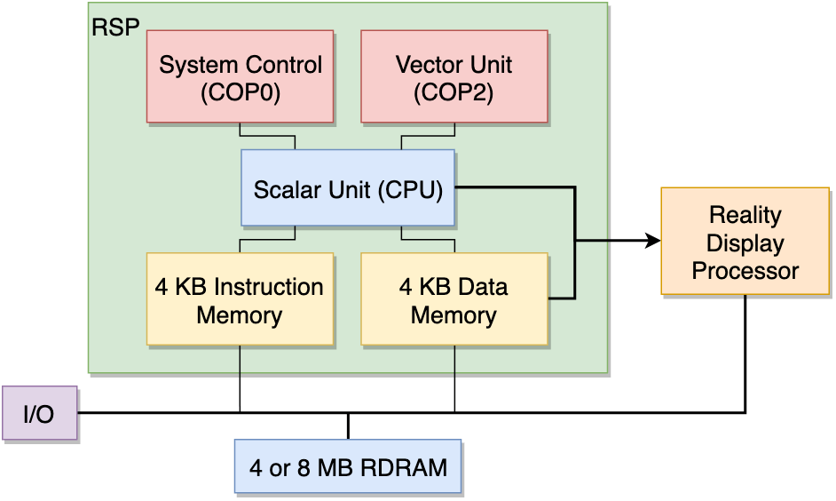
I think there is: a sub-component called the Reality Signal Processor (RSP), with the architecture shown in the figure below, courtesy of Rodrigo Copetti.
The RSP is essentially another CPU package, with a scalar unit, which I believe is the manager of the RSP, and Vector Unit which is does the bulk of the compute.
The vector unit does operations with 32 128-bit registers, where each register is sliced into eight parts to process eight 16-bit vectors at once.
If used correctly for our DNNs, we could potentially get some pretty high speedups thanks to the parallelism that SIMD unit provides.
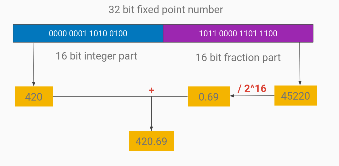
The main CPU of the N64 has a floating point unit (FPU), but we don’t have floating point number support in the RSP’s vector unit.
That means if we want to approximate the float numbers typically used in DNNs, we’ll need to use fixed point numbers.
In this case, that would be 16 bits for the integer part, and 16 bits for the fractional part.
An example of that is shown in the figure below.
That might not be ideal for DNNs, where most of our values are between 0 and 1 anyway.
This is what motivated the creation of the bfloat16 data-type.
Alternatively, we could look at quantizing our DNNs to use integers, but we can leave that for another post.
Example of a 32-bit fixed point number, with 16 bits for the integer part and 16 bits for the fractional part
Additionally, the RSP has 4KB of instruction cache, and 4KB of data cache.
So if we want to use this to accelerate our DNNs, we need to think carefully about how and when we copy data to and from the RSP.
We’ll look into this issue in a future post - for now it will be okay to run our DNN using the main CPU of the N64.
If you’re interested in the topic of data movement to-and-from DNN accelerators, I’d recommend the AXI4MLIR paper, which I co-authored.
When developing this project, I’ll be using an emulator, which is a software program that emulates the hardware of the N64 on another machine, e.g., my laptop.
Ideally there should be no difference between the real hardware and the emulator, but there are always some differences.
For now, it is sufficient for development, but I’ll need to test on real hardware before I can say that I’ve succeeded in my project.
Apache TVM
Now we have some more information about the hardware we’re deploying to, we can think about how we can get our DNNs running on it.
I mentioned Apache TVM earlier, which is a tensor compiler which can take DNN models from a variety of sources (e.g., PyTorch, TensorFlow, ONNX), and generate efficient code for a range of platforms, including Arm, Intel, and RISC-V CPUs; Arm, AMD, and NVidia GPUs; OpenCL, CUDA, LLVM, and Vulkan software backends; and more.
I’ll discuss more of how TVM works as required in this post series, but check out its excellent docs and tutorials if you’re interested in learning more.
The question is how can we use TVM to generate our code for the N64?
We could export to LLVM, and then go to our MIPS backend from there.
But since C is a bit more hackable for a single person, and we have a C toolchain already to go, why not do that?
Fortunately, TVM has a backend for that too: MicroTVM.
Originally intended for deployment in microcontrollers, MicroTVM can generate C code, which can then be deployed using whatever a given microcontroller requires.
It generates C, with the rationale that almost everything has at least a C compiler.
This tutorial is the most pertinent to our deployment requirements, since it generates C code directly, rather than trying to integrate with a known toolchain.
If we untar the file it genrates, we should have all of the code we need to execute our model, including the model definition, weights, and runtime.
We will need to tweak the code generation a bit later, but for now this has taken us a long way.
Note that I also considered the Darknet framework, a DNN framework written in C.
But since it isn’t a compiler, it means we would include a lot of unused functions if our DNN doesn’t use every single layer type it supports, and we lose a lot of potential optimizations (e.g., loop unrolling) by not knowing our shapes ahead-of-time.
The combination of libdragon and TVM
Two things we need are integration of our TVM model code with our libdragon build system, and a way to automatically generate our inference management code (i.e., our main function).
The generated TVM code should be relatively self-contained, though still requires some standard library functions.
My go-to for these kind of projects is usually CMake, but I elected to stick to a Makefile, since libdragon already provided a pretty decent build config for our target backend, and I didn’t want to try porting it over.
There isn’t much more to say about the build system: anyone that’s had to wrangle a build system for a new project will tell you it can be annoying, and once the core is set up, don’t poke it too much.
It works, and that’s what matters.
For our main function, we need to be able to:
Load some sample data for our target model
Load and execute our target model with the sample data
Fetch the output, and compare it against our target output
Print any info or debug messages that will help us understand the execution
We could hardcode this for every model that we want to deploy, but that’s not very compiler-brained — our programs should write themselves.
The approach I’ve gone for is to use the Jinja templating engine, typically used for generating HTML files, in frameworks such as Flask, I’m using it for C, defining a main.c.template file for our project, which we populate as required.
By using the double brace syntax {{my_var}}, we can define substitutions that can be placed in our code by the templating engine.
Sidenote: multiple braces can be valid C syntax, which could cause us problems. So far, my template doesn’t have any, so the point is moot, but another syntax might be better for larger systems).
We could have a template like:
#include<libdragon.h>#include"tvm/runtime/crt/platform.h"
#include"tvmgen_default.h"
#include<math.h>{{samples_import}}intmain(void){{{target_outputs}}{{output_dtype}}actual_output;{{output_dtype}}expected_outputs[{{num_outputs_to_check}}];inputs.{{input_name}}=(void*)&{{sample_name0}};// rest of the code}
We can then use Jinja to fill in these fields with ones relevant to our target model.
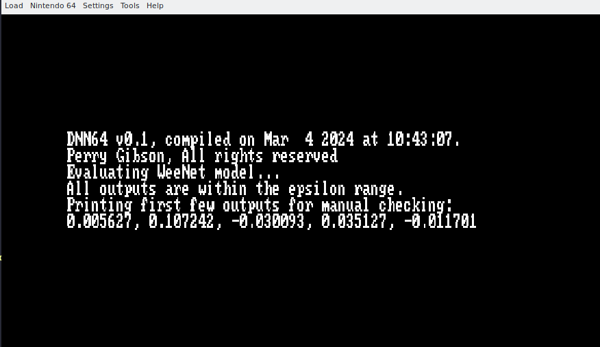
With our build system and main function ready, we can compile our a small test model, and execute it on an N64 emulator.
Here it is!
First run of a DNN on the N64
Conclusions and acceleration challenges
This post briefly introduces the workflow I’m using for DNN64.
With just a bit of elbow grease, we can get DNNs running on the N64!
But there’s still work to do.
We are especially limited by the 4MB memory of the N64, so there are lots of optimizations we’ll need to apply to get non-trivial models working.
This includes changes to our code generation, quantisation, and understanding how the graphics accelerator of the N64 can be exploited.
We’ll talk about those in future posts, as well as going deeper into my code which I will be open sourcing.
For now, catch ye.
]]>Perry Gibson 🍐Press: HiPEAC Info 712024-02-16T11:00:00+00:002024-02-16T11:00:00+00:00https://gibsonic.org/blog/2024/02/16/press_hipeac
I’m pleased to say that I have been featured in issue 71 of the HiPEAC Info magazine, available here from the HiPEAC website. You can find it on pages 48-49. During the interview with a HiPEAC team member, I had the opportunity to discuss my PhD journey, share some of the techniques I developed, and offer insights that could be beneficial to current and prospective PhD candidates.
]]>Perry Gibson 🍐How to Instantly Open Files at Specific Positions in KDE Konsole2024-01-21T12:00:00+00:002024-01-21T12:00:00+00:00https://gibsonic.org/blog/2024/01/21/opening_files_from_konsole
I often use KDE Konsole for running terminal commands, but sometimes I’m using a tool (e.g., a compiler) which outputs a file path, as well as a line number, which I may want to open in my text editor. E.g.,
2 errors generated.
In file included from /home/proj/lib/AsmParser/Parser.cpp:13:
/home/proj/include/mlir/IR/MLIRContext.h:253:18: error: use of undeclared identifier 'Operation'; did you mean 'operator'?
Wouldn’t it be handy if we could just click on/select the file in the terminal output, and open it in our text editor in the right place?
This would reduce friction when debugging, potentially increasing productivity.
This isn’t default behaviour in Konsole, however with a very small amount of configuration we can allow it.
At time of writing, I’m using Konsole Version 22.12.3, so these steps may have changed slightly for you.
First thing you need to do is open your Konsole configuration panel (Settings->Configure Konsole, or Ctrl+Shift+,).
Our solution is configured on a per-profile basis, so select the profile you want to edit (probably your default profile), and click “Edit”.
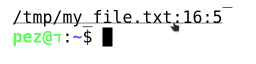
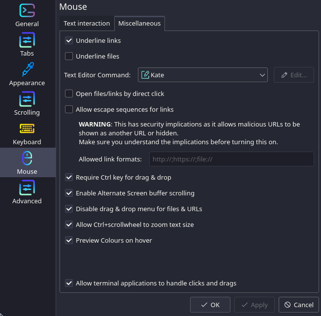
Next, select Mouse on the left panel, and then select Miscellaneous ribbon at the top (see screenshot below):
Next, you should select the “Underline files” option, as well as the “Open files/links by direct click”.
Finally, edit the “Text Editor Command” to match your text editor of choice.
For me, it had to be Custom, as there’s some additional arguments I needed to configure.
Editing the default command (which should look something like kate PATH:LINE:COLUMN), we see some documentation of the variables we have available:
The format is e.g. ‘editorExec PATH:LINE:COLUMN’
PATH will be replaced by the path to the text file
LINE will be replaced by the line number
COLUMN (optional) will be replaced by the column number Note: you will need to replace ‘PATH:LINE:COLUMN by the actual syntax the editor you want to use supports; e.g.:
gedit +LINE:COLUMN PATH
If PATH or LINE aren’t present in the command, this setting will be ignored and the file will be opened by the default text editor.
For me, that is emacsclient +LINE:COLUMN -n PATH.
Apply, and exit, and our desired behaviour should now be available!
]]>Perry Gibson 🍐Step-by-step Guide to Adding a New Dialect in MLIR2024-01-11T12:00:00+00:002024-01-11T12:00:00+00:00https://gibsonic.org/blog/2024/01/11/new_mlir_dialect
For one of my projects, I needed to add a new dialect to the main MLIR tree.
However, following the information available, I encountered some issues.
I made a “clean” example dialect, which I was able to add correctly.
This post discusses how this is achieved, and links to some code.
The information in this post was sourced partially from Chapter 2 of the Toy tutorial and Creating a Dialect tutorial.
I hope to update the latter with some of the steps described below.
Note that MLIR/LLVM often has API breaking changes, and this guide may not by entirely correct or best practice when reading.
My code builds on 42204c9.
The first thing we need to do is decide how we want to define our dialect.
MLIR allows us to define the dialect using TableGen, which automatically generates a lot of the boilerplate required, as well as reducing the costs of maintenance if an API breaking change occurs.
We could also write the C++ ourselves, but for many dialects this is overkill.
Step 1: Let’s create a directory mlir/include/mlir/Dialect/Foo/, where we will store our dialect definitions.
Make sure to add_subdirectory(Foo) in the CMakeLists.txt of mlir/include/mlir/Dialect.
Step 2: Next, we’re going to define the basic definition of our dialect, mlir/include/mlir/Dialect/Foo/FooBase.td.
Here’s we’ll give our dialect a name, the C++ namespace that it will use, and a description:
#ifndef FOO_BASE
#define FOO_BASE
include "mlir/IR/OpBase.td"
def Foo_Dialect : Dialect {
  let name = "foo";
  let cppNamespace = "::mlir::foo";
  let description = [{
    Lorem Ipsum
  }];
}
#endif // FOO_BASE
Step 3: Let’s also create a mostly blank file FooOps.td.
This is where we would include the definition of the operations of our dialect, if we had any.
For now, let’s just put some simple includes:
#ifndef FOO_OPS
#define FOO_OPS

include "mlir/Dialect/Foo/FooBase.td"
include "mlir/Interfaces/InferTypeOpInterface.td"
include "mlir/Interfaces/VectorInterfaces.td"
include "mlir/Interfaces/SideEffectInterfaces.td"

#endif // FOO_OPS
These two files will generate some C++ files that can be included elsewhere in the project.
For example, in our build directory (once we’ve set up the rest of our code), we will generate the file ./tools/mlir/include/mlir/Dialect/Foo/FooOps.h.inc.
This will look something like this, actually defining the C++ class of our dialect.
Note that the above is automatically generated, and you should only edit the TableGen files to create it.
You can extend the dialect with C++ later if you want, or for some advanced cases you may need to define your dialect in C++ from the start.
Step 4: I also defined a file Foo.h, which we can use to include our dialect elsewhere, avoiding the ugliness of .inc files.
This looks like:
Step 6: Finally, an optional step is to ensure that our dialect is registered globally, otherwise we will need to add it to the registry of whatever tool we need it for manually.
If you open the file mlir/include/mlir/InitAllDialects.h, you will see where this is done.
Add the lines #include "mlir/Dialect/Foo/Foo.h", and foo::FooDialect, to the registry.insert call, and once we’re finished the dialect should be globally available.
You can put a registry.insert line for your dialect in the executable you care about if you don’t want it registered globally.
Source code
There isn’t much regarding “implementation” for our dialect, since we don’t actually have any operations or transformations yet.
However to get our minimum working dialect, we do require a little bit of code.
Step 7: First, let’s create a Foo directory in mlir/lib/Dialect/Foo/.
Be sure to add add_subdirectory(Foo) to the CMakeLists.txt of the parent directory.
Next, let’s create a file FooDialect.cpp.
This will use some of auto-generated implementation boilerplate from the previous steps, see the #include statements.
Step 8: Finally, let’s create our CMakeLists.txt.
This will create the dialect library, and allow us to link against other executables.
It should also make the library available under the CMake variable dialect_libs, which is used in the compilation of tools such as mlir-opt.
Thus you won’t need to do any manual linking to get that working.
Great, we now have everything we need to compile, creating our new dialect Foo, and registering it in the main MLIR dialect registry.
Go ahead and build.
Now, to verify that our dialect was added correctly, we can run mlir-opt.
Pass the --show-dialects and it will give a list of loaded dialects.
You should see foo amongst them.
And that’s us done.
You can extend this example to make a more fully featured dialect.
Now you have a working dialect, now might be the time to revisit the dialect definition tutorial.
Bonus! Adding an operation
Clearly, the next step to creating a dialect is to start adding operations to it!
You can see in the Toy tutorial how we can do that, but what does this look like in our stripped down Foo dialect?
We defined an initial FooOps.td ODS file above, but we didn’t actually include any operations.
Let’s update this file:
include "mlir/Dialect/Foo/FooBase.td"
include "mlir/Interfaces/FunctionInterfaces.td"
include "mlir/IR/SymbolInterfaces.td"
include "mlir/Interfaces/SideEffectInterfaces.td"

class Foo_Op<string mnemonic, list<Trait> traits = []> :
    Op<Foo_Dialect, mnemonic, traits>;

def BarOp : Foo_Op<"bar"> {
    let summary = "bar operation";
}
We define a high-level Foo_Op, which all of the operations in our Foo dialect are derived from.
Then, we have our operation, which we will call bar.
Right now it takes not arguments and returns nothing, and we have our definition under BarOp.
Much like before, TableGen will create the necessary header files and implementations for our operation.
The other thing we need to add is the appropriate inclusion of our op classes.
Add the following to the end of our FooDialect.cpp file:
This uses the same stack that big Sean Cosgrove and I used for the “Bloodshot” music video, as seen in DJ Magazine and this blogpost.
Happy holidays to aw yoos.
]]>Perry Gibson 🍐Google Project Management: Professional Certificate2023-12-12T12:00:00+00:002023-12-12T12:00:00+00:00https://gibsonic.org/blog/2023/12/12/mooc_google_project_management
In this post, I am pleased to announce that I have received a certificate for completing the Google Project Management course, comprised of six modules over six months.
Although I have gained significant experienced in managing projects during my time at gicLAB, as well as my other professional endeavours, I felt that re-familiarising myself with the terminology and best practices of the field would serve me well.
You can find my certificate of completion here.
Outcomes: I was able to apply these skills for developing grant proposals during my time at gicLAB.
I was instrumental in developing gicLAB’s contribution to the dAIedge consortium application to the EU, which was awarded over 14 million euros. I applied techniques from the course to ensure that our planned contributions were achievable and well document.
I elected to not continue with a post-doc with gicLAB, and thus had to plan out the project in more detail for a new start. This required me translating a lot of my institutional and project knowledge into additional documentation to help them. For example, a stakeholder management plan, and a more detailed task breakdown.