DNN64: An ML Compiler Toolchain for the Nintendo 64 (Part 4) --- The Co-Processor
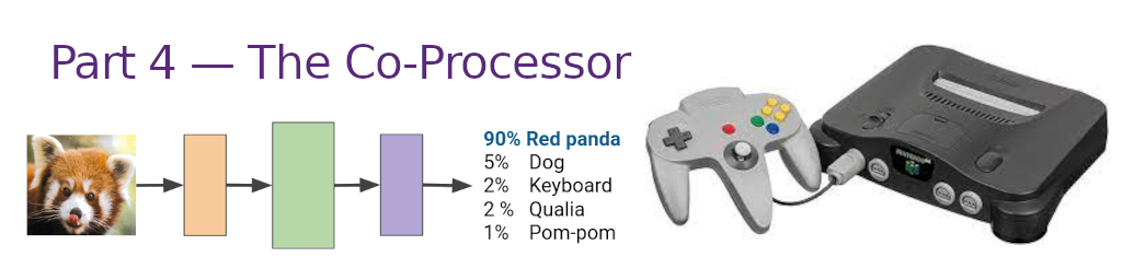
This post is the fourth in my DNN64 series, where I discuss my project of compiling and accelerating deep neural networks (DNNs) on the Nintendo 64 system using modern tools and techniques. My first post is available here, and the goal is to use modern tools and techniques on this constrained platform. This post discusses the N64’s co-processor, the RSP, which I am using to accelerate my DNN computations.
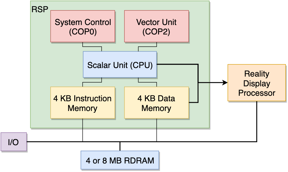
The N64’s RSP (Reality Signal Processor) was kind of ahead of its time as a graphics processor. Although other machines were beginning to include dedicated chips for graphics acceleration, the RSP stood apart as being truly general purpose. By that, I mean that instead of processing using a small set of fixed functions, it has a full instruction set programmed using assembly. Its acceleration came from the vector unit, which is a MIPS core with vector instructions (128-bit lanes, with each of the 8 lanes being 16-bits wide). There is also a scalar unit which can execute simultaneously (assuming there aren’t data hazards), although its instruction set is significantly reduced.
One of the reasons why the project is appealing to me is that this high-level system design, of a CPU with a co-processor with more limited memory, is very similar to modern DNN accelerator environments (CPU+GPU/TPU/etc). Therefore, many of the design decisions and trade-offs that we will make on this “old” platform are similar to the kind of ones we might make in modern ones. Namely, how do we fit computations that are too large onto it, balancing the performance considerations of the cost of sending and receiving data, and the fact that we can do work on the CPU at the same time.
Sure, the N64 hardware is old, but these are the same problems I’ve faced in others works using modern hardware, e.g., the SECDA project (led by the talented hardware systems designed Jude Haris). Moreover, we’re using modern software tooling, so the retro nature of the N64 is almost irrelevant, it’s just in terms of resources it’s now closer to the a contemporary micro-controller.
Kicking it 90s style
One of the first steps I took when looking into this accelerator was to rtfm, if you can believe it. The RSP manual is available here, released in 1996, which I used to both gain some insights into the RSP’s design and behaviour; as well as some historical interest.
Let’s take a couple of excepts that stood out to me, more on an aesthetic level than a technical one:
For example:
Mastery of the information presented in this document will occur slowly, as the information is both voluminous and of tremendous breadth. Some concepts, such as the hardware architecture of the RSP and the microcode assembly language, are of course thoroughly intertwined; discussion of one is impossible without the other.
Youch, that doesn’t bode well!
Standing alone, the RSP is an extremely powerful processor; a fixed-point RISC CPU capable of over half a billion arithmetic operations per second![1] As part of the RCP, the RSP is an integral part of the graphics/audio/video processing pipelines. Recommended background for this chapter includes a solid foundation in computer architecture, including RISC processors and SIMD (Single Instruction, Multiple Data) machines.
[1] This is not a misprint. At 62.5Mhz with an 8-element vector pipeline, the RSP could perform 500,000,000 multiply-accumulate operations per second. Since the RSP dual-issues scalar instructions, you could also do another 62,500,000 scalar operations during that same second. That is more than three times the performance of the Cray supercomputers from twenty years ago.
Half a billion arithmetic operations per second! Can you believe it. For reference, 2019’s NVidia 3090 can do like five orders of magnitude more! Although to be fair, both the RSP and the 3090 leave my ability to do mental maths in the dust
This next quote gives information about performance optimization of RSP programs, but also highlights the main designer of the RSP was someone called Mary Jo Doherty.
Mary Jo’s Rules [1]
Avoiding pipeline stalls in software can be accomplished by understanding the following rules.
- VU register destination writes 4 cycles later (need 3 cycles between load and use). This applies to vector computational instructions, vector loads, and coprocessor 2 moves (mtc2).
- SU register load takes 3 cycles (need 2 cycles between load and use). This applies to SU loads and coprocessor moves (mfc0, cfc2, mfc2). SU computational results are available in the next cycle (see “SU is Bypassed” on page 44).
- ny load followed by any store 2 cycles later, causes a one cycle bubble. Coprocessor moves (mtc0, mfc0, mtc2, mfc2, ctc2, cfc2) count as both loads and stores.
- branch target not 64-bit aligned always single issues.
- ranches: a. Can dual issue (with preceding instruction). b. o branch instruction permitted in a delay slot. c. elay slot always single issues. d. Taken branch causes a 1 cycle bubble.
[1] Named after Mary Jo Doherty, the designer of the RSP.
She seems to have a had a pretty illustrious career, at organisations such as Silicon Graphics (where the RSP was developed), Sun Microsystems, Transmeta Corporation, Digital Equipment Corporation, Oracle, and SambaNova. Cheers Mary Jo!
Finally, for you hardware-heads, here’s some concise info:
The RSP has a vector processor, implemented as MIPS Coprocessor. The vector unit (VU) has 32 128-bit wide vector registers (which can also be accessed as 8 vector slices), a vector accumulator (which also has 8 vector slices), and several special-purpose vector control registers. The VU instruction set includes all useful computational instructions (add, multiply, logical, reciprocal, etc.) plus additional “multimedia instructions” which are well suited for graphics and audio processing. These instructions are thoroughly explained in Chapter 3, “Vector Unit Instructions”.
Pipeline depth varies among MIPS processors and their implementations. The RSP has a pipeline depth of 5.
As discussed earlier, the RSP is programmed in assembly, and with a decent enough manual like this, it should be possible to get our accelerated DNN layers implemented this way. However, writing assembly can be time consuming, and optimizing it has the issue of making it very difficult to parse, especially after multiple passes of optimization strategies like instruction reordering. In principle, I could write this assembly myself, like my forebears did, but I’m not sure if this is the kind of guy I want to become.
This is one of the many motivations for using a compiler — write your code in a more readable high-level language, and let the compiler handle the generation and optimization of the assembly.
Since LLVM can generate MIPS code, I considered making some alterations specifically for the RSP. However, this ended up not being necessary because I found as of October 2023, someone is making a DSL (domain-specific language) and optimising compiler for the RSP: RSPL!
RSPL: Really Saves Perry’s Lardon 🥓
I’ve been building up a repository of examples of RSPL, which I’ve released under an MIT License on my GitHub. I’ll discuss some of these examples more in a future post when I talk about accelerating DNN computations.
You can see some annotated examples below, which I encourage you to copy-paste into the RSPL web-app to see the assembly it generates. Experiment with turning optimization and re-ordering on and off to see its impact:
Add one to a list of 8 values
state
{
  // Allocate space for our data
  vec16 DATA[1];
}

command<0> AddOne(u32 addrData)
{
  // first byte of first arg has metadata
  // that needs to be dropped
  addressMatC &= 0xFFFFFF;

  // Perform DMA from CPU into RSP mem
  dma_in(DATA, addrData);

  // vec16 is a vector type, with 8 16-bit elements
  // Here we load from RSP mem into a vector register
  vec16 d = load(DATA, 0x00);

  d += 1; // Add one to every element (SIMD instruction)

  // Store register in RSP mem
  store(d, DATA, 0x00);

  // Return data to CPU over DMA
  dma_out(DATA, addrData);
}
Reduction of a list of 8 values (sum is stored in idx 0)
command<0> Reduction(u32 addressMatC)
{
  addressMatC &= 0xFFFFFF;

  // Perform DMA for input
  dma_in(INPUT, addressMatC);

  // Load value into register
  vec16 psum = load(INPUT, 0x00);

  // Use swizzle syntax to get sum
  // first value is the sum, rest are junk
  psum += psum.yywwYYWW;
  psum += psum.zzzzZZZZ;
  psum += psum.X;
  store(psum, INPUT, 0x00);

  dma_out(INPUT, addressMatC);
}
Conclusions
This post gave a quick overview of the Reality Signal Processor (RSP), the main accelerator in the N64. We discussed a little bit about its architecture (128-bit 8 lane vector instructions), as well as how we can program it. Future posts will discuss how we can accelerate DNN computations using it.